Sequential Refinement of
Small Angle Scattering Data
In
this tutorial you will fit USAXS small angle scattering data for “Ludox” colloidal silica (Aldrich, LUDOX TM-50?) prepared in
a range of dilutions to demonstrate the sequential refinement technique in
GSAS-II for SASD and demonstrate fitting with a hard sphere structure factor
for non-dilute systems.
If you have not done so already, start GSAS-II.
Step 1: read in the data files
1. Use the Import/Small Angle Data/from q (A-1) step X-ray QIE data file menu item to read the data files into GSAS-II. This read option is set to read three column small angle scattering data (SASD) as Q in Å-1, intensity and estimated standard deviation in intensity; there may be a header with metadata information in the front of this file. It will read multiple files from a single directory. Change the file directory to SAseqref/data to find the files.
2. Select the six data files with ‘Ludox’ in their name in the first dialog and press Open. All six will immediately be read into GSAS-II; you will have to select the any file (*.*) filter to see them.
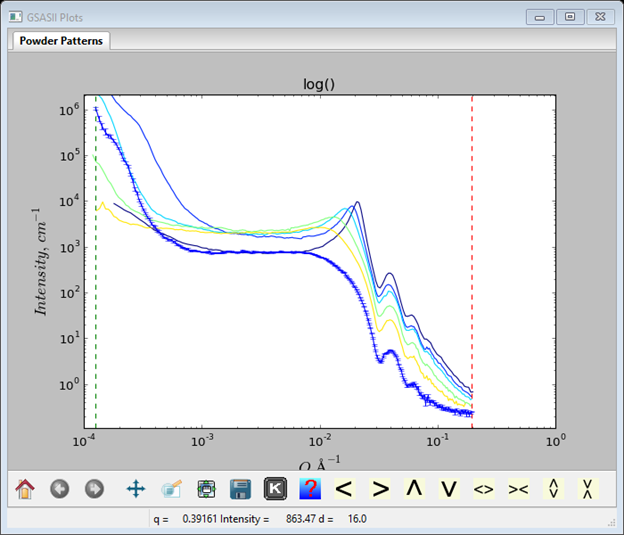
At this point the GSAS-II data tree window will have several entries and the plot window will show the SASD pattern for one as a log-log plot of intensity vs. Q; enter ‘m’ on the plot. Now all are shown; one shows error bars (SASD S49_Ludox6_1pct.dat) as it is the selected tree entry and the others as lines.
Step 2: Set Limits
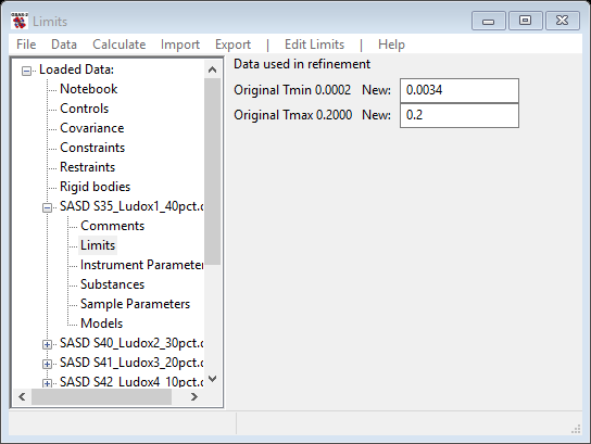
For this step we will reposition the limits to exclude the low-Q (<10-3) part of the patterns which do not seem to follow the sequence evident in the 10-2 – 10-1 part. Select Limits under SASD S35_Ludox1_40pct.dat from the GSAS-II tree. Set the lower limit using the cursor on the plot by picking a point somewhere in the flat region at Q~3x10⁻³ with the left mouse button. The limits window should look something like
To copy these limits to the other data sets use the Edit
Limits/Copy command from the data window menu; a popup window will
give the selection of targets.
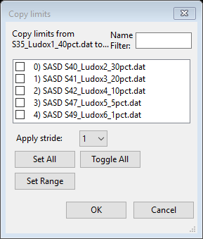
Do Set All (all boxes will be checked) and then press OK to do the copy.
Step 3 Select the scattering substances for your sample
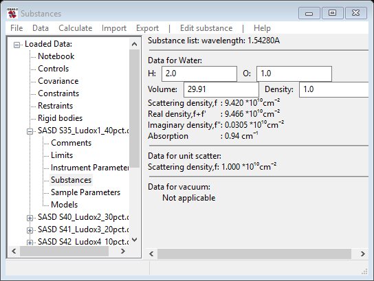
Two substances need to be defined for your sample to give the anticipated scattering contrast; in this case one is silica and the other is water. Parameters for a number of substances are defined in the file Substances.py. You can add your own substances to this or better put them in UserSubstances.py; this is read after Substances.py when you load substances for your selection. Select Substances from the GSAS-II tree. Then do Edit substance/Load substance from the menu; a popup window will appear with possible selections
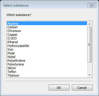
Notice that silica is not one of the choices; we will add it in a moment (a-Quartz is but let’s ignore that). Select Water and press OK; the relevant data for water (and vacuum) are displayed next
If desired, you can load/add as many substances as you want to this list; you can also delete any of them (except vacuum or unit scatter). The composition, volume occupied by the atoms in the composition and the density are given for each substance. These can each be edited; the other values will change accordingly. Since we are going to say that silica wasn’t in the list of known substances, do Edit substance/Add substance to create it; you will be asked for a name – enter silica and then a periodic table of the elements will be shown. Select Si and O

They appear in red. Press OK and silica will be added to your substance list
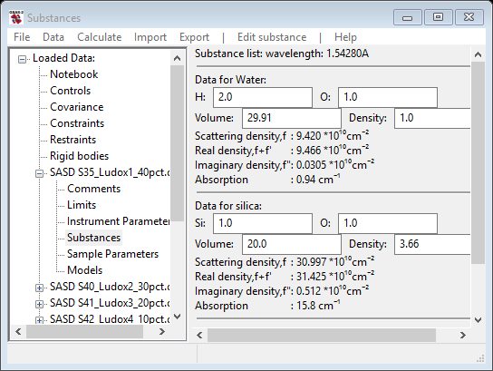
Change the O-atom entry to 2.0 and the density to 2.65, on the section of data for silica; the window will change each time giving new values and should finally show

From this information the scattering density and that as affected by resonant scattering for the listed wavelength is displayed (the wavelength can be changed in the Instrument Parameters GSAS-II tree item if needed). The real density value is used for contrast calculations.
Just as for Limits, this information needs to be copied to the other SASD entries in the GSAS-II tree. Do Edit substance/Copy substances from the data window menu and follow the same selection procedure as you used for limits above.
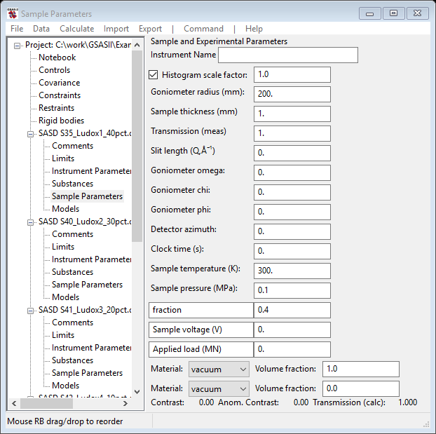
Step 4: Set Sample parameters
As these data sets were
collected from a sequence of samples where there was some variable changed in
their preparation, it would be useful to have this information available to
GSAS-II for subsequent analysis. Select Sample parameters from the data tree.
It shows (for SASD S49_Ludox6_1pct.dat)
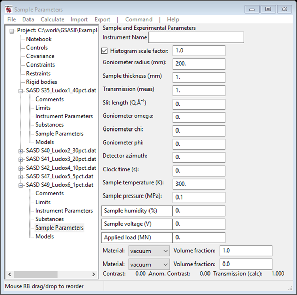
NB: we will not be needing to
select the Material for this analysis; material selection is only
required for Size distribution analysis. Notice that the last three column names can
be changed; pick the first one and change it to fraction. Then enter 0.01 which corresponds to the ‘1pct’ in the file name. The data window should look like
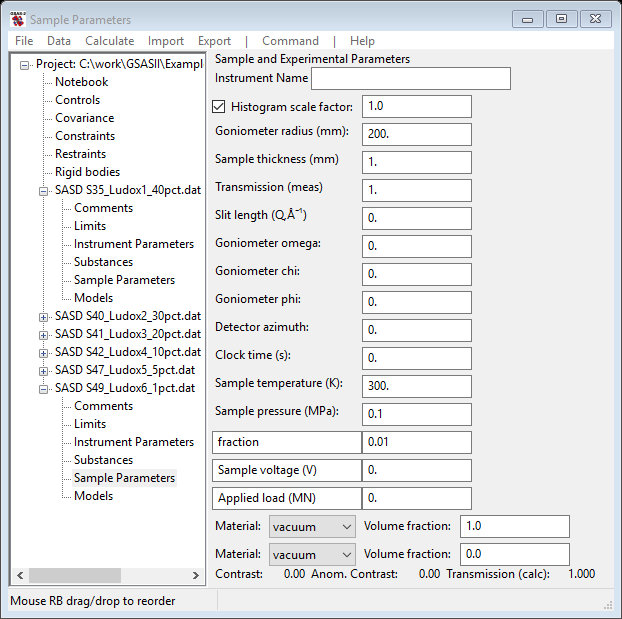
Now do the same for the Sample Parameters for the other data sets putting in the correct fraction from the respective file names. If you first Copy this one to the others, that will save you the step of changing the names. You will end up on the Sample parameters page for SASD S35_Ludox1_40pct.dat GSAS-II data tree.
Step 5: Set Model parameters
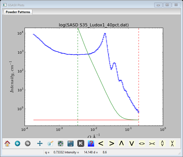
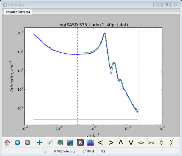
Looking at the data plot (key ‘m’ to select a single data set) for SASD S35_Ludox1_40pct.dat, one sees just one feature with oscillations at higher Q. This is the signal for a non-dilute scatterer.

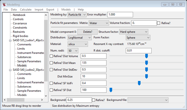
Select Models from the GSASII data tree under SASD S35_Ludox1_40pct.dat, switch Size dist. to Particle fit, and add a reasonable value (0.25) for the Background; a horizontal red line will appear. Next do Models/Add; the window will display a default component; change the Material to silica. Also change the Matrix to Water; the calculated contrast should be 175.60 1020cm-4. The plot will show a green curve corresponding to the default values.
The default Dist Mean of 1e+03 is too large, try something smaller and increase the Dist Volume (the sliders work well for this). Since this is a non-dilute system, change the Structure factor to Hard sphere and set the SF VolFr to 0.4. Your data window should look something like
And the plot will be
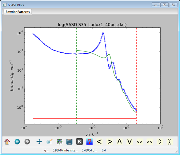
The calculated curve shows oscillations but they are not in the right place and are too broad. Try the Dist StdDev slider and make it smaller; somewhere about 0.132 gives a curve with the right shape but too high. Reduce the Dist Volume to improve the match. Shift the SF Dist and SF VolFr as well to get the curves to match. Carefully manipulate each of the sliders to see what effect they have on the calculated curve. With some adjustments I got

to give a pretty nice initial fit.
Step 6: Initial refinement
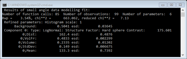
We can be brave and set all six Refine? boxes (NB: the one for Matrix Volume fraction currently does not operate – ignore it). Then do Models/Fit; the least squares very quickly minimizes to give

The console window lists the results
And the plot shows the fit graphically

The fit is OK except for a region Q~0.03Å-1; this is probably due to a failure of the simple hard sphere model in this concentrated system.
Step 7: Sequential refinement
We are now ready to try a sequential refinement starting with this fit for the 1st data set. Do Models/Sequential fit; a dialog box will appear for selection of the data sets.
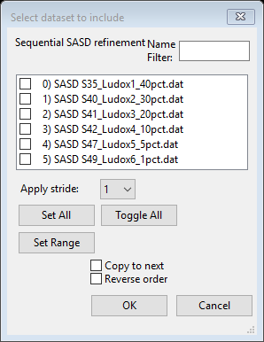
Press Set All,
all boxes will be checked showing selection of the data sets. This also allows
you to instruct the sequential refinement to start at the last data set and
proceed backwards through them (Reverse order). It also allows you
to instruct the sequential refinement to use the current parameters as starting
values for the next data set. This works in either direction and facilitates
the initial sequential refinements. NB: some sequential refinements do not work
well in both directions; in this particular case starting with a fitted 1%
pattern and going in reverse through the data fails on the 5% data set.
Apparently the change in parameters is too great for the least squares to
handle; going in the forward direction works just fine (as you will see next).
Select Copy to next
and press OK;
the sequential refinement will proceed very rapidly displaying results for each
data set on the console and finally ending by displaying the Sequential refinement
results.
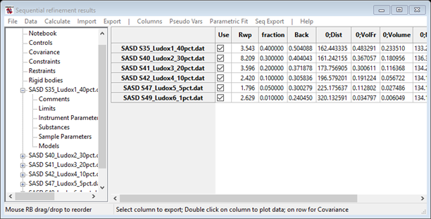
Note the comment in the plot status bar: double click on the 0;Volume and a new plot will appear.

Each point has an error bar extracted from the least squares – it represents a 1 σ variation in the value. Now press the s key (or select s from the K box); a dialog box will appear with a selection of parameters to plot along the x-axis. Select fraction and the plot will be redrawn (it may require selection of another column & then 0;Volume to make it appear).
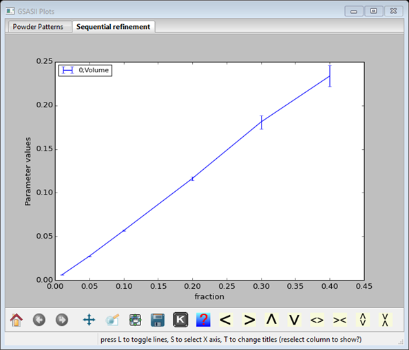
It is gratifying how this relation between Volume and the composition is linear. You can now determine the slope & intercept (or fit to some other function!) directly with GSAS-II; do Parametric Fit/Add equation and the Expression Editor dialog box will appear.

The pull down in the upper left corner has two choices; select Global and a new dialog box will appear giving you choices from the Sequential results table. Select 0;Volume and the Expression Editor will reappear.

Next enter the function you wish to use in fitting 0:Volume; enter m*x+b (equation for a straight line). After a pause, the Expression Editor will be redrawn allowing you to assign b, m & x.

For b & m select Free; these will be the parameters for your fit. For x select Global; a new dialog box will appear giving you several choices.
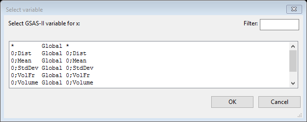
Select the last line (fraction…); it will appear in blue. Then press OK; the Expression Editor will reappear with more information.

Next press OK; the equation will be fitted to the data and the results displayed on the console
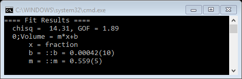
And the plot shows the curve (in red) calculated from the best fit, weighted by the esds on the data points, to the model equation for a straight line.

For this particular experiment there was an expectation that the Volumes obtained from the SASD model fits would match the makeup concentrations for these samples so that the slope for this plot would be unity. One possible explanation for the discrepancy is that the silica particles are partially hydrated thus reducing the contrast from 175.6x1020 cm-4 to something like 98x1020cm-4. This concludes the small angle sequential fit tutorial; you may save the project.